8U CubeSat Thermal Analysis
Demonstration of the missiontools thermal tools.
Scenario
8U CubeSat (10 × 20 × 40 cm, 1×2×4U configuration)
500 km sun-synchronous orbit, nadir-pointed
All six faces radiate to space
Internal electronics dissipate 5 W continuously
Cryocooler keeps an IR detector at cryogenic temperatures
Environmental heat loads (computed automatically per face):
Direct solar absorption
Earth albedo (reflected sunlight, default albedo = 0.3)
Earth infrared emission (default 240 W/m²)
We model three thermal nodes: the main bus (structure + electronics), a radiator panel, and an IR detector cooled by an active cooler.
[1]:
import numpy as np
import matplotlib.pyplot as plt

from missiontools import Spacecraft, NormalVectorThermalConfig
from missiontools.attitude import FixedAttitudeLaw
from missiontools.thermal import ThermalCircuit
1. CubeSat geometry and orbit
Body frame convention (nadir pointing): body-z = nadir, body-x = along-track. The 40 cm long axis is along body-z (nadir).
[2]:
# Orbit
EPOCH = np.datetime64('2025-03-20T12:00:00', 'us')  # spring equinox

sc = Spacecraft.sunsync(
    altitude_km=500.0,
    node_solar_time='10:30',
    epoch=EPOCH,
)
sc.attitude_law = FixedAttitudeLaw.nadir(0.0)

mu = sc.central_body_mu
period_s = 2 * np.pi * np.sqrt(sc.a**3 / mu)

print(f'Altitude        : 500 km')
print(f'Inclination     : {np.degrees(sc.i):.2f}°')
print(f'LTAN            : 10:30')
print(f'Orbital period  : {period_s / 60:.1f} min')
Altitude        : 500 km
Inclination     : 97.40°
LTAN            : 10:30
Orbital period  : 94.6 min
2. Surface thermal model
All six faces of the cubesat are modelled as thermal surfaces. Each face has a solar absorptivity and an IR emissivity determined by its surface finish.
The NormalVectorThermalConfig automatically computes three environmental heat loads for each face based on its orientation:
Direct solar: absorbed when the face sees the Sun (zero in eclipse)
Earth IR: absorbed proportionally to the face’s view factor to Earth (uses emissivity by Kirchhoff’s law)
Earth albedo: reflected sunlight from Earth, proportional to the face’s view factor and the solar illumination of the sub-satellite point
[3]:
# Face definitions: (normal, area_m2, emissivity, absorptivity)
faces = {
    'Nadir (+Z)':       ([0, 0,  1], 0.10 * 0.20, 0.80, 0.30),
    'Zenith (-Z)':      ([0, 0, -1], 0.10 * 0.20, 0.80, 0.30),
    '+X (along-track)': ([1, 0,  0], 0.20 * 0.40, 0.85, 0.25),
    '-X (anti-track)':  ([-1, 0, 0], 0.20 * 0.40, 0.85, 0.25),
    '+Y side':          ([0, 1,  0], 0.10 * 0.40, 0.90, 0.20),  # radiator face
    '-Y side':          ([0, -1, 0], 0.10 * 0.40, 0.90, 0.20),
}

normals       = np.array([f[0] for f in faces.values()], dtype=float)
areas         = np.array([f[1] for f in faces.values()])
emissivities  = np.array([f[2] for f in faces.values()])
absorptivities = np.array([f[3] for f in faces.values()])

print(f"{'Face':<22} {'Normal':>14} {'Area (cm\u00b2)':>11} {'\u03b5':>5} {'\u03b1':>5}")
print('-' * 60)
for name, (n, a, e, al) in faces.items():
    print(f'{name:<22} {str(n):>14} {a * 1e4:>8.1f}    {e:.2f}  {al:.2f}')
print(f"{'Total':<22} {'':>14} {areas.sum() * 1e4:>8.1f}")
Face                           Normal  Area (cm²)     ε     α
------------------------------------------------------------
Nadir (+Z)                  [0, 0, 1]    200.0    0.80  0.30
Zenith (-Z)                [0, 0, -1]    200.0    0.80  0.30
+X (along-track)            [1, 0, 0]    800.0    0.85  0.25
-X (anti-track)            [-1, 0, 0]    800.0    0.85  0.25
+Y side                     [0, 1, 0]    400.0    0.90  0.20
-Y side                    [0, -1, 0]    400.0    0.90  0.20
Total                                   2800.0
[4]:
thermal_cfg = NormalVectorThermalConfig(
    normal_vecs=normals,
    areas=areas,
    emissivities=emissivities,
    absorptivities=absorptivities,
    # earth_ir=240.0,  # W/m², default
    # albedo=0.3,      # default
)
sc.add_thermal_config(thermal_cfg)

print(f'Thermal config: {thermal_cfg.num_faces} faces attached to spacecraft')
print(f'Earth IR flux : {thermal_cfg.earth_ir} W/m²')
print(f'Earth albedo  : {thermal_cfg.albedo}')
Thermal config: 6 faces attached to spacecraft
Earth IR flux : 240.0 W/m²
Earth albedo  : 0.3
3. Thermal circuit
Three thermal nodes:
bus: main structure + electronics (aluminium, ~2 kg equivalent thermal mass)
radiator: dedicated radiator panel on +Y face (aluminium sheet, ~0.1 kg)
detector: IR detector (small thermal mass, actively cooled)
The bus dissipates 5 W from electronics. A cryocooler pumps heat from the detector to the radiator.
[5]:
circuit = ThermalCircuit()

# Thermal capacitances  (C = m × c_p;  aluminium c_p ≈ 900 J/(kg·K))
circuit.add_capacitance('bus',      2.0 * 900,  initial_temp=293.0)  # 2 kg
circuit.add_capacitance('radiator', 0.1 * 900,  initial_temp=293.0)  # 0.1 kg
circuit.add_capacitance('detector', 0.02 * 900, initial_temp=293.0)  # 0.02 kg

# Thermal resistances (K/W)
circuit.connect('bus', 'radiator', 0.5)    # good conductive path
circuit.connect('bus', 'detector', 5.0)    # weak thermal link (isolation)

# Internal heat sources
circuit.add_heat_source('electronics', 5.0, target='bus')

# Active cooler: extracts heat from detector, rejects to radiator
circuit.add_cooler(
    'cryo', cold_node='detector', hot_node='radiator',
    power=1.5,       # 1.5 W electrical input
    efficiency=0.15,  # 15% of Carnot COP
    cop_max=5.0,
)

print(circuit)
ThermalCircuit(nodes=3, sources=1, coolers=1, connections=2)
4. Couple surfaces to circuit and solve
Each face is assigned to a thermal node:
Nadir, zenith, ±X, −Y faces → bus
+Y face → radiator
We simulate 3 orbits (~285 minutes) to see the periodic thermal response.
[6]:
# Map each face to a circuit node
face_nodes = ['bus', 'bus', 'bus', 'bus', 'radiator', 'bus']
#              nadir  zenith  +X     -X     +Y          -Y

n_orbits = 3
t_start = EPOCH
t_end   = EPOCH + np.timedelta64(int(n_orbits * period_s * 1e6), 'us')

duration = thermal_cfg.attach(
    circuit,
    face_nodes=face_nodes,
    t_start=t_start,
    t_end=t_end,
    step=np.timedelta64(30, 's'),
)

print(f'Simulation duration: {duration / 60:.1f} min ({n_orbits} orbits)')
print(f'Solving thermal circuit...')

t_eval = np.linspace(0, duration, 2000)
result = circuit.solve(duration, t_eval=t_eval)

print(f'Done. Solver success: {result.success}')
Simulation duration: 283.8 min (3 orbits)
Solving thermal circuit...
Done. Solver success: True
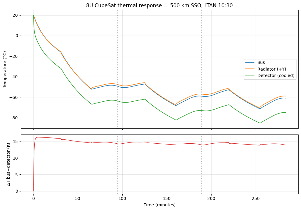
5. Results
[7]:
t_min = result.t / 60  # convert to minutes

fig, (ax1, ax2) = plt.subplots(2, 1, figsize=(10, 7), sharex=True,
                                height_ratios=[2, 1])

# Temperature plot
ax1.plot(t_min, result.temperatures['bus'] - 273.15,
         linewidth=1.2, label='Bus', color='tab:blue')
ax1.plot(t_min, result.temperatures['radiator'] - 273.15,
         linewidth=1.2, label='Radiator (+Y)', color='tab:orange')
ax1.plot(t_min, result.temperatures['detector'] - 273.15,
         linewidth=1.2, label='Detector (cooled)', color='tab:green')

# Mark orbital period boundaries
for k in range(1, n_orbits):
    ax1.axvline(k * period_s / 60, color='grey', linestyle=':', alpha=0.5)

ax1.set_ylabel('Temperature (\u00b0C)')
ax1.set_title('8U CubeSat thermal response \u2014 500 km SSO, LTAN 10:30')
ax1.legend(loc='right')
ax1.grid(True, alpha=0.3)

# Temperature difference: bus − detector
delta_T = result.temperatures['bus'] - result.temperatures['detector']
ax2.plot(t_min, delta_T, linewidth=1.0, color='tab:red')
ax2.set_xlabel('Time (minutes)')
ax2.set_ylabel('\u0394T bus\u2212detector (K)')
ax2.grid(True, alpha=0.3)
for k in range(1, n_orbits):
    ax2.axvline(k * period_s / 60, color='grey', linestyle=':', alpha=0.5)

plt.tight_layout()
plt.show()
[8]:
# Summary statistics (last orbit)
last_orbit = result.t > (n_orbits - 1) * period_s

print('=' * 55)
print('Thermal summary \u2014 last orbit (quasi-steady state)')
print('=' * 55)
print(f"{'Node':<15} {'Min (\u00b0C)':>10} {'Max (\u00b0C)':>10} {'Mean (\u00b0C)':>10} {'\u0394T (K)':>10}")
print('-' * 55)
for name in ['bus', 'radiator', 'detector']:
    T = result.temperatures[name][last_orbit]
    T_c = T - 273.15
    print(f'{name:<15} {T_c.min():>10.1f} {T_c.max():>10.1f} {T_c.mean():>10.1f} {T_c.max() - T_c.min():>10.1f}')
=======================================================
Thermal summary — last orbit (quasi-steady state)
=======================================================
Node              Min (°C)   Max (°C)  Mean (°C)     ΔT (K)
-------------------------------------------------------
bus                  -71.3      -52.7      -61.5       18.6
radiator             -70.5      -51.2      -60.1       19.3
detector             -85.2      -67.3      -75.7       17.9