Canada Coverage Analysis

End-to-end demonstration of missiontools coverage and plotting features, using a rectangular (pushbroom-style) sensor.

Scenario

• Sun-synchronous orbit, 550 km, 10:30 LTAN (ascending)

• Nadir-pointed rectangular sensor, 5° cross-track × 30° along-track half-angles

• Min ground elevation: 20°

• Illumination constraint: solar zenith angle < 70° (daytime)

• Area of interest: Canada (20 000 km² point density)

• Simulation window: 90 days

import numpy as np
import matplotlib.pyplot as plt
import cartopy.crs as ccrs

from missiontools import Spacecraft, RectangularSensor, AoI, Coverage
from missiontools.plotting import plot_ground_track, plot_coverage_map

1. Build the spacecraft

EPOCH = np.datetime64('2025-05-01T00:00:00', 'us')

sc = Spacecraft.sunsync(
    altitude_km=550.0,
    node_solar_time='10:30',
    epoch=EPOCH,
)

print(f"Semi-major axis : {sc.a/1e3:.1f} km")
print(f"Inclination     : {np.degrees(sc.i):.2f} deg")
print(f"RAAN            : {np.degrees(sc.raan):.2f} deg")
print(f"Propagator      : {sc.propagator_type}")

Semi-major axis : 6928.1 km
Inclination     : 97.59 deg
RAAN            : 15.96 deg
Propagator      : j2

2. Attach a nadir-pointed rectangular sensor

RectangularSensor models a pyramidal FOV defined by two independent half-angles in orthogonal planes. Here we use a narrow cross-track half-angle (10°) with a wider along-track half-angle (30°), modelling a pushbroom imager.

sensor = RectangularSensor(
    theta1_deg=10.0,
    theta2_deg=30.0,
    body_vector=[0, 0, 1],
)
sc.add_sensor(sensor)

print(f"Cross-track half-angle : {sensor.theta1_deg:.1f}°")
print(f"Along-track half-angle : {sensor.theta2_deg:.1f}°")

Cross-track half-angle : 10.0°
Along-track half-angle : 30.0°

3. Define the Area of Interest

aoi = AoI.from_geography('Canada', point_density=20_000)
print(f"AoI sample points: {len(aoi)}")

AoI sample points: 644

4. Set up Coverage analysis

cov = Coverage(
    aoi,
    [sensor],
    el_min_deg=20.0,
    sza_max_deg=70.0,
)

5. Run the 90-day simulation

T_START = EPOCH
T_END   = EPOCH + np.timedelta64(90 * 24 * 3600, 's')

print("Computing coverage fraction ...")
frac = cov.coverage_fraction(T_START, T_END, max_step=np.timedelta64(10, 's'))
print(f"  Final cumulative coverage : {frac['final_cumulative']:.1%}")
print(f"  Mean instantaneous        : {frac['mean_fraction']:.1%}")

print("\nComputing revisit times ...")
rev = cov.revisit_time(T_START, T_END, max_step=np.timedelta64(10, 's'))

Computing coverage fraction ...
  Final cumulative coverage : 100.0%
  Mean instantaneous        : 0.0%

Computing revisit times ...

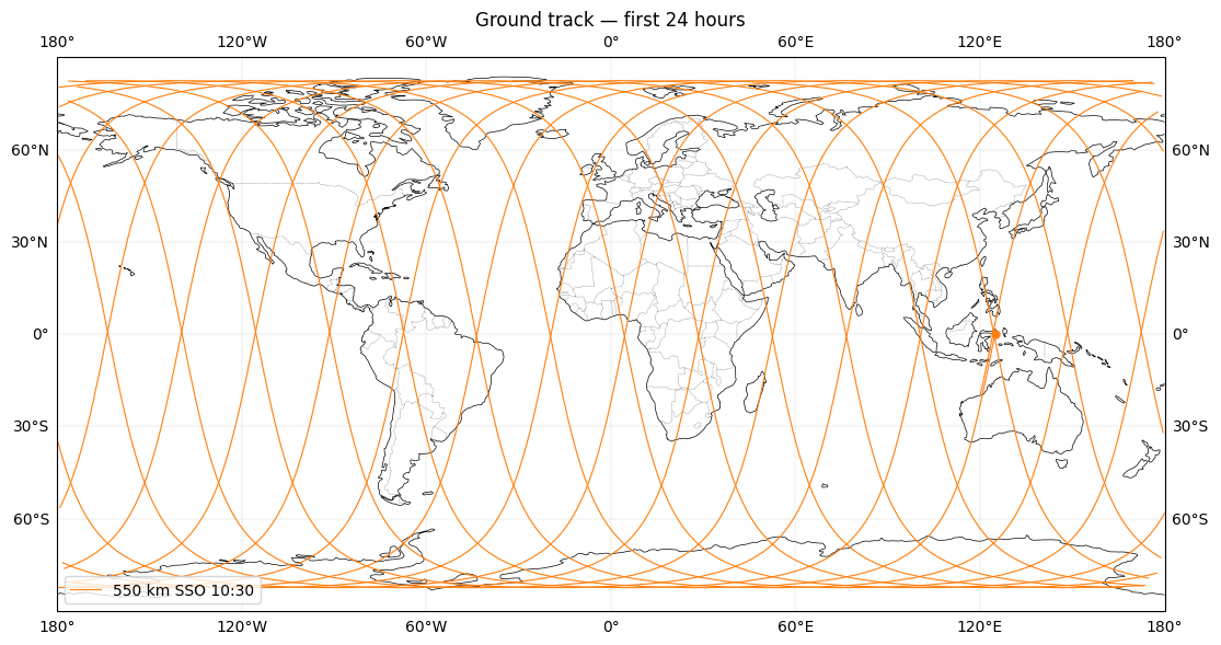
6. Ground track — first 24 hours

fig = plt.figure(figsize=(14, 6))
ax  = fig.add_subplot(1, 1, 1, projection=ccrs.PlateCarree())

plot_ground_track(
    sc,
    T_START,
    T_START + np.timedelta64(24 * 3600, 's'),
    ax=ax,
    color='tab:orange',
    label='550 km SSO 10:30',
    linewidth=0.8,
)
ax.set_title('Ground track — first 24 hours')
ax.legend(loc='lower left')
plt.tight_layout()
plt.show()

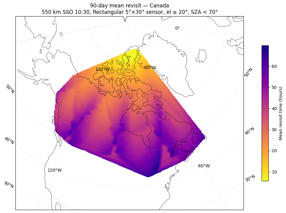
7. Coverage maps over Canada

We use a Lambert Conformal Conic projection with the same geometric parameters as EPSG:3347 (Statistics Canada Lambert). We define it manually because Cartopy’s ccrs.epsg(3347) carries restrictive area-of-use bounds from the EPSG registry that clip southern Canada out of the renderable area.

canada_proj = ccrs.LambertConformal(
    central_longitude=-91.867,
    central_latitude=63.391,
    standard_parallels=(49, 77),
)

mean_rev_hrs = rev['mean_revisit'] / 3600.0

fig, ax = plt.subplots(
    figsize=(12, 7),
    subplot_kw={'projection': canada_proj},
)
plot_coverage_map(
    aoi,
    mean_rev_hrs,
    ax=ax,
    auto_window=True,
    cmap='plasma_r',
    colorbar_label='Mean revisit time (hours)',
    title='90-day mean revisit — Canada\n550 km SSO 10:30, Rectangular 5°×30° sensor, el ≥ 20°, SZA < 70°',
)
plt.tight_layout()
plt.show()

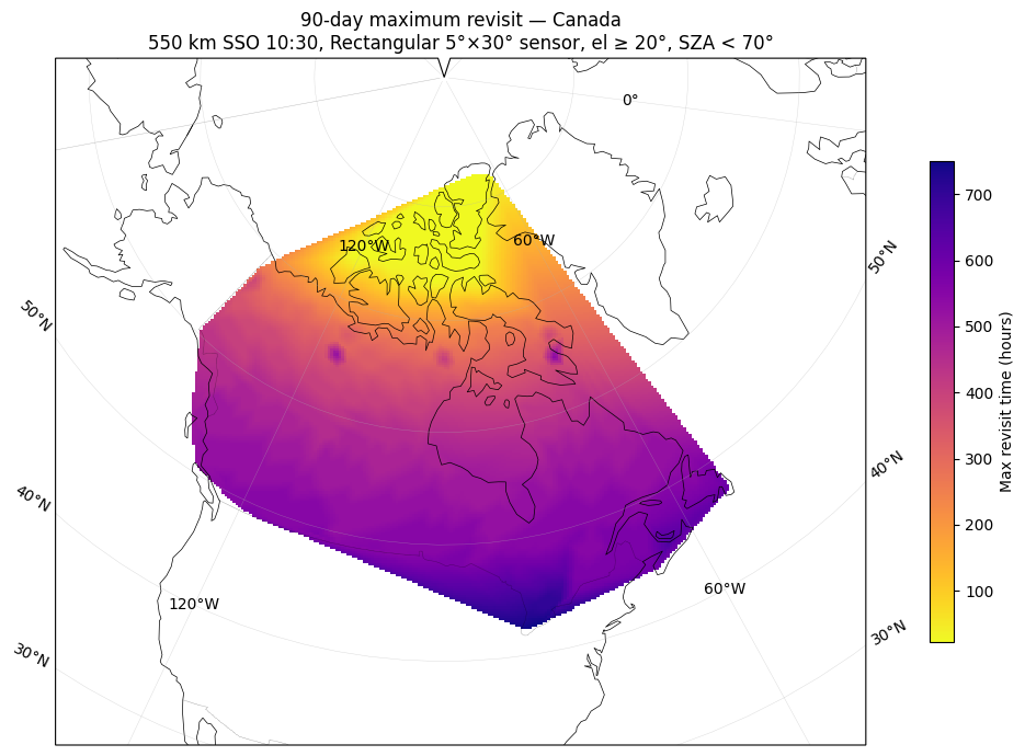
max_rev_hrs = rev['max_revisit'] / 3600.0

fig, ax = plt.subplots(
    figsize=(12, 7),
    subplot_kw={'projection': canada_proj},
)
plot_coverage_map(
    aoi,
    max_rev_hrs,
    ax=ax,
    auto_window=True,
    cmap='plasma_r',
    colorbar_label='Max revisit time (hours)',
    title='90-day maximum revisit — Canada\n550 km SSO 10:30, Rectangular 5°×30° sensor, el ≥ 20°, SZA < 70°',
)
plt.tight_layout()
plt.show()

8. Summary statistics

print("=" * 55)
print("90-day coverage summary — Canada")
print("550 km SSO 10:30 | Rectangular 5°×30° sensor")
print("=" * 55)
print(f"Cumulative coverage fraction : {frac['final_cumulative']:.1%}")
print(f"Mean instantaneous coverage  : {frac['mean_fraction']:.1%}")
print()
global_mean_hrs = rev['global_mean'] / 3600.0
global_max_hrs  = rev['global_max']  / 3600.0
print(f"Global mean revisit time     : {global_mean_hrs:.1f} h")
print(f"Global max revisit time      : {global_max_hrs:.1f} h")

=======================================================
90-day coverage summary — Canada
550 km SSO 10:30 | Rectangular 5°×30° sensor
=======================================================
Cumulative coverage fraction : 100.0%
Mean instantaneous coverage  : 0.0%

Global mean revisit time     : 40.5 h
Global max revisit time      : 750.4 h