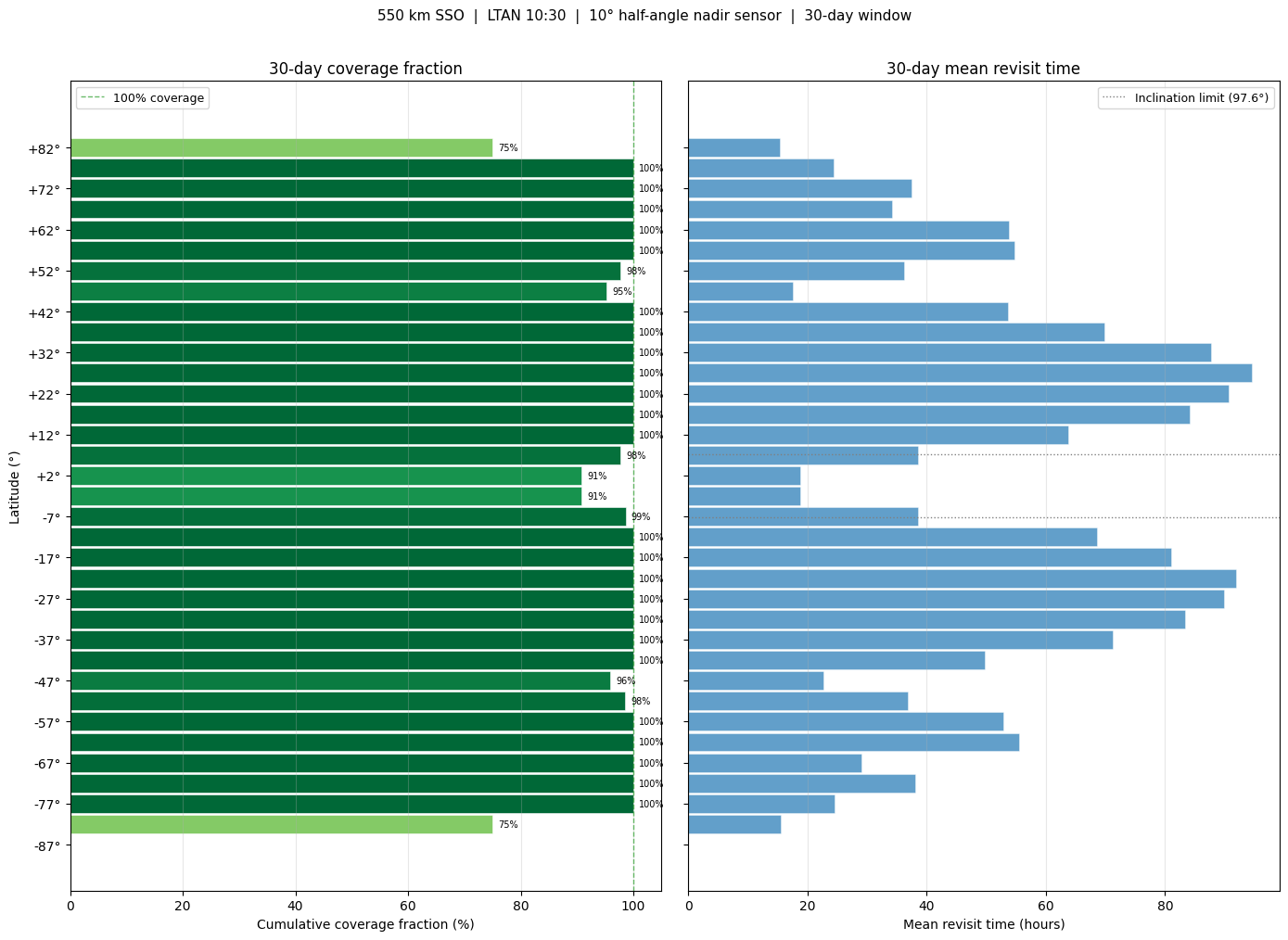
SSO Coverage by Latitude Band
Computes 30-day coverage statistics for a 550 km sun-synchronous orbit (LTAN 10:30, descending node) carrying a 10° half-angle nadir sensor.
Results are reported per 5° latitude band:
Number of sample points in the band
Cumulative coverage fraction (% of points seen ≥ once)
Mean revisit time (hours)
Maximum revisit time (hours)
Object API — uses Spacecraft.sunsync, Sensor, AoI.from_region, and Coverage.
[1]:
import time
import numpy as np
import matplotlib.pyplot as plt
import matplotlib.colors as mcolors

from missiontools import Spacecraft, Sensor, AoI, Coverage
1. Spacecraft and Sensor
A nadir-pointing 10° half-angle sensor is body-mounted along the spacecraft nadir axis (body-z = nadir, body-vector [0, 0, 1] in the sensor convention).
[2]:
EPOCH = np.datetime64('2025-01-01T00:00:00', 'us')

sc = Spacecraft.sunsync(
    altitude_km    = 550.0,
    node_solar_time = '10:30',
    node_type      = 'descending',
    epoch          = EPOCH,
)

sensor = Sensor(half_angle_deg=10.0, body_vector=[0, 0, 1])
sc.add_sensor(sensor)

period_s = 2 * np.pi * np.sqrt(sc.a**3 / sc.central_body_mu)
swath_km = 2 * (sc.a - sc.central_body_radius) * np.tan(np.radians(10.0)) / 1e3

print(f"Semi-major axis : {sc.a / 1e3:.1f} km")
print(f"Inclination     : {np.degrees(sc.i):.3f}°")
print(f"Orbital period  : {period_s / 60:.1f} min")
print(f"Propagator      : {sc.propagator_type}")
print(f"FOV half-angle  : {np.degrees(sensor.half_angle_rad):.0f}°")
print(f"Ground swath    : ~{swath_km:.0f} km")
Semi-major axis : 6928.1 km
Inclination     : 97.593°
Orbital period  : 95.6 min
Propagator      : j2
FOV half-angle  : 10°
Ground swath    : ~194 km
2. Per-Band Coverage Analysis
For each 5° latitude band we create an AoI.from_region, attach a fresh Coverage object, and compute coverage fraction and revisit time.
Note — 36 bands × 30 days takes a few minutes.
[3]:
T_START = EPOCH
T_END   = EPOCH + np.timedelta64(30 * 86_400, 's')

MAX_STEP     = np.timedelta64(20, 's')
POINT_DENSITY = 200_000   # km²/point  (~450 km resolution)

LAT_EDGES = np.arange(-90, 91, 5)   # 37 edges → 36 bands

def band_label(lo_deg, hi_deg):
    lo_s = f"{abs(lo_deg):.0f}°{'S' if lo_deg <  0 else 'N'}"
    hi_s = f"{abs(hi_deg):.0f}°{'S' if hi_deg <= 0 else 'N'}"
    return f"{lo_s} – {hi_s}"

rows = []   # (label, n_pts, cov_pct, mean_rev_h, max_rev_h)

t0 = time.perf_counter()

for lo_deg, hi_deg in zip(LAT_EDGES[:-1], LAT_EDGES[1:]):
    aoi = AoI.from_region(
        lat_min_deg = float(lo_deg),
        lat_max_deg = float(hi_deg),
        point_density = POINT_DENSITY,
    )
    n = len(aoi)

    cov = Coverage(aoi, [sensor])

    cf = cov.coverage_fraction(T_START, T_END, max_step=MAX_STEP)
    rt = cov.revisit_time(T_START, T_END, max_step=MAX_STEP)

    cov_pct    = cf['final_cumulative'] * 100.0
    mean_rev_h = rt['global_mean'] / 3600.0 if not np.isnan(rt['global_mean']) else float('nan')
    max_rev_h  = rt['global_max']  / 3600.0 if not np.isnan(rt['global_max'])  else float('nan')

    rows.append((band_label(lo_deg, hi_deg), n, cov_pct, mean_rev_h, max_rev_h))

elapsed = time.perf_counter() - t0
print(f"Done in {elapsed:.1f} s")
Done in 151.3 s
3. Coverage Table
[4]:
print(f"  {'Band':>13}  {'Pts':>5}  {'Coverage':>10}  {'Mean Rev':>10}  {'Max Rev':>10}")
print(f"  {'─'*13}  {'─'*5}  {'─'*10}  {'─'*10}  {'─'*10}")

for label, n, cov_pct, mean_rev_h, max_rev_h in rows:
    mean_s = f"{mean_rev_h:8.2f} h" if not np.isnan(mean_rev_h) else "       —  "
    max_s  = f"{max_rev_h:8.2f} h" if not np.isnan(max_rev_h)  else "       —  "
    print(f"  {label:>13}  {n:>5}  {cov_pct:>9.1f}%  {mean_s}  {max_s}")
           Band    Pts    Coverage    Mean Rev     Max Rev
  ─────────────  ─────  ──────────  ──────────  ──────────
    90°S – 85°S      9        0.0%         —           —
    85°S – 80°S     28       75.0%     15.49 h    113.24 h
    80°S – 75°S     48      100.0%     24.58 h    588.37 h
    75°S – 70°S     65      100.0%     38.04 h    533.89 h
    70°S – 65°S     84      100.0%     29.01 h    629.53 h
    65°S – 60°S    100      100.0%     55.47 h    515.14 h
    60°S – 55°S    118      100.0%     52.80 h    583.17 h
    55°S – 50°S    132       98.5%     36.87 h    702.71 h
    50°S – 45°S    148       95.9%     22.69 h    705.03 h
    45°S – 40°S    160      100.0%     49.80 h    705.04 h
    40°S – 35°S    173      100.0%     71.24 h    609.43 h
    35°S – 30°S    184      100.0%     83.34 h    513.82 h
    30°S – 25°S    194      100.0%     89.96 h    464.93 h
    25°S – 20°S    201      100.0%     91.86 h    536.63 h
    20°S – 15°S    208      100.0%     81.06 h    608.33 h
    15°S – 10°S    213      100.0%     68.57 h    680.03 h
     10°S – 5°S    216       98.6%     38.60 h    703.92 h
      5°S – 0°S    218       90.8%     18.79 h     59.74 h
      0°N – 5°N    218       90.8%     18.74 h     59.74 h
     5°N – 10°N    216       97.7%     38.58 h    703.92 h
    10°N – 15°N    213      100.0%     63.73 h    680.02 h
    15°N – 20°N    208      100.0%     84.18 h    608.33 h
    20°N – 25°N    201      100.0%     90.64 h    536.63 h
    25°N – 30°N    194      100.0%     94.49 h    464.93 h
    30°N – 35°N    184      100.0%     87.71 h    513.82 h
    35°N – 40°N    173      100.0%     69.86 h    609.42 h
    40°N – 45°N    160      100.0%     53.66 h    681.12 h
    45°N – 50°N    148       95.3%     17.60 h     58.58 h
    50°N – 55°N    132       97.7%     36.29 h    702.71 h
    55°N – 60°N    118      100.0%     54.78 h    583.18 h
    60°N – 65°N    100      100.0%     53.87 h    515.14 h
    65°N – 70°N     84      100.0%     34.27 h    658.59 h
    70°N – 75°N     65      100.0%     37.55 h    533.89 h
    75°N – 80°N     48      100.0%     24.46 h    580.18 h
    80°N – 85°N     28       75.0%     15.33 h    170.54 h
    85°N – 90°N      9        0.0%         —           —
4. Visualisation
[5]:
labels    = [r[0] for r in rows]
lat_mids  = [(lo + hi) / 2 for lo, hi in zip(LAT_EDGES[:-1], LAT_EDGES[1:])]
cov_pcts  = np.array([r[2] for r in rows])
mean_revs = np.array([r[3] for r in rows])
max_revs  = np.array([r[4] for r in rows])

# Colour bars by coverage fraction
norm    = mcolors.Normalize(vmin=0, vmax=100)
cmap    = plt.cm.RdYlGn
colours = [cmap(norm(v)) for v in cov_pcts]

fig, (ax1, ax2) = plt.subplots(1, 2, figsize=(14, 10), sharey=True)

# --- Coverage fraction ---
ax1.barh(lat_mids, cov_pcts, height=4.5, color=colours, edgecolor='white', linewidth=0.4)
ax1.axvline(100, color='tab:green', linestyle='--', linewidth=1.0, alpha=0.7, label='100% coverage')
ax1.set_xlabel('Cumulative coverage fraction (%)')
ax1.set_ylabel('Latitude (°)')
ax1.set_title('30-day coverage fraction')
ax1.set_xlim(0, 105)
ax1.set_yticks(lat_mids[::2])
ax1.set_yticklabels([f"{int(l):+d}°" for l in lat_mids[::2]])
ax1.grid(True, axis='x', alpha=0.3)
ax1.legend(fontsize=9)

# Add value labels
for lat, v in zip(lat_mids, cov_pcts):
    if v > 0:
        ax1.text(min(v + 1, 103), lat, f"{v:.0f}%", va='center', fontsize=7)

# --- Mean revisit time ---
valid = ~np.isnan(mean_revs)
ax2.barh(np.array(lat_mids)[valid], mean_revs[valid], height=4.5,
         color='tab:blue', alpha=0.7, edgecolor='white', linewidth=0.4)
ax2.set_xlabel('Mean revisit time (hours)')
ax2.set_title('30-day mean revisit time')
ax2.grid(True, axis='x', alpha=0.3)

# Inclination limit annotation
ax2.axhline(np.degrees(sc.i) - 90, color='grey', linestyle=':', linewidth=1.0,
            label=f'Inclination limit ({np.degrees(sc.i):.1f}°)')
ax2.axhline(-(np.degrees(sc.i) - 90), color='grey', linestyle=':', linewidth=1.0)
ax2.legend(fontsize=9)

fig.suptitle(
    f'550 km SSO  |  LTAN 10:30  |  10° half-angle nadir sensor  |  30-day window',
    fontsize=11, y=1.01
)
plt.tight_layout()
plt.show()